Anomaly Detection in Semiconductor Manufacturing

Deep Learning for Wafer Map Defect Classification

WaferGuardML

2026-03-26

Agenda

1. Background — Why semiconductor defect detection matters
2. Key Concepts — Neural networks, CNNs, transfer learning explained
3. Dataset & Exploration — The wafer map dataset
4. Data Preprocessing — Encoding, splitting, augmentation
5. Phase 1 — Multi-label classification (8 defect types)
6. Phase 2 — Multi-class classification (38 defect patterns)
7. Results & Evaluation
8. Visual Representation

Walk through the agenda briefly. Emphasize that the first section is a primer for non-technical audience members.

Why Semiconductor Defect Detection?

• Semiconductor chips are in everything — phones, cars, medical devices
• During manufacturing, silicon wafers go through hundreds of process steps
• Defects on the wafer surface cause chip failures
• Traditional inspection: manual review by engineers — slow, subjective, expensive
• Our goal: automate defect pattern recognition using deep learning

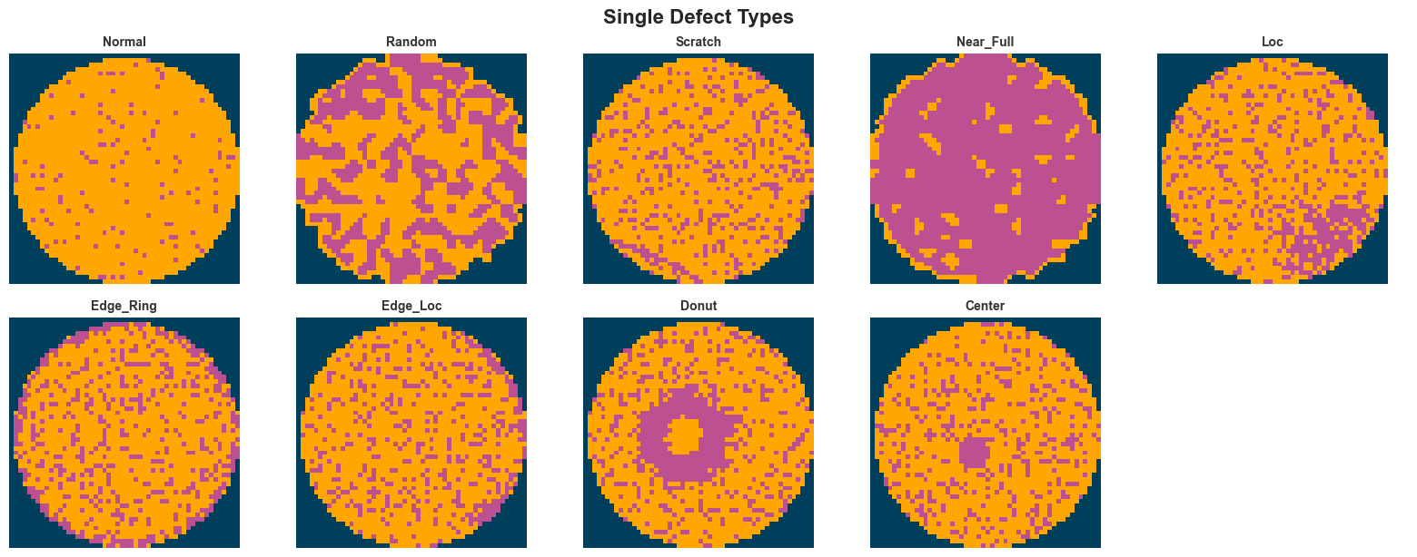
The 8 Base Defect Types

Explain that a wafer is a thin slice of silicon, and each small square on it becomes a chip. Defects = bad chips = money lost.

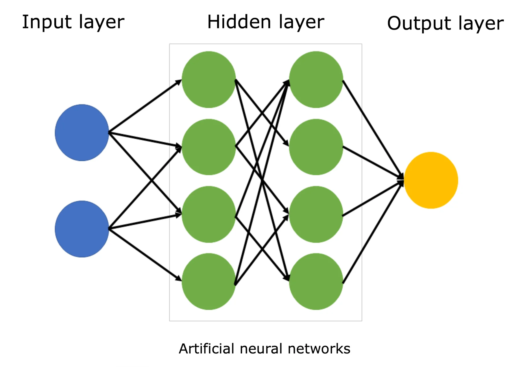
What is a Neural Network?

Think of it as a decision-making system inspired by the brain:

• Inputs: Raw data (e.g., pixel values of a wafer image)
• Hidden layers: Each layer learns to detect increasingly complex patterns
• Output: A prediction (e.g., “this wafer has a scratch defect”)

The network learns by example — we show it thousands of labeled wafer images, and it figures out what patterns correspond to each defect type.

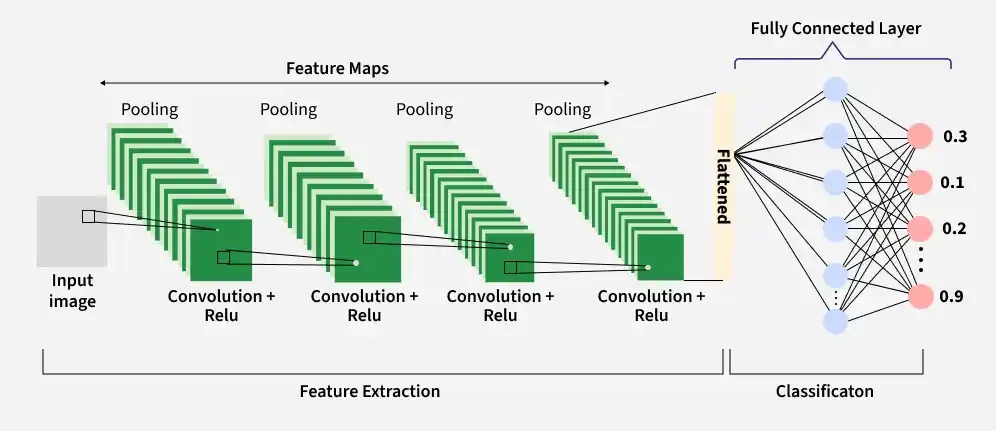
What is a Convolutional Neural Network (CNN)?

A CNN is a specialized neural network designed for images.

Why CNN for wafer maps? Defect patterns are spatial — a “ring” defect forms a circle, a “scratch” forms a line. CNNs are built to detect exactly these kinds of spatial structures.

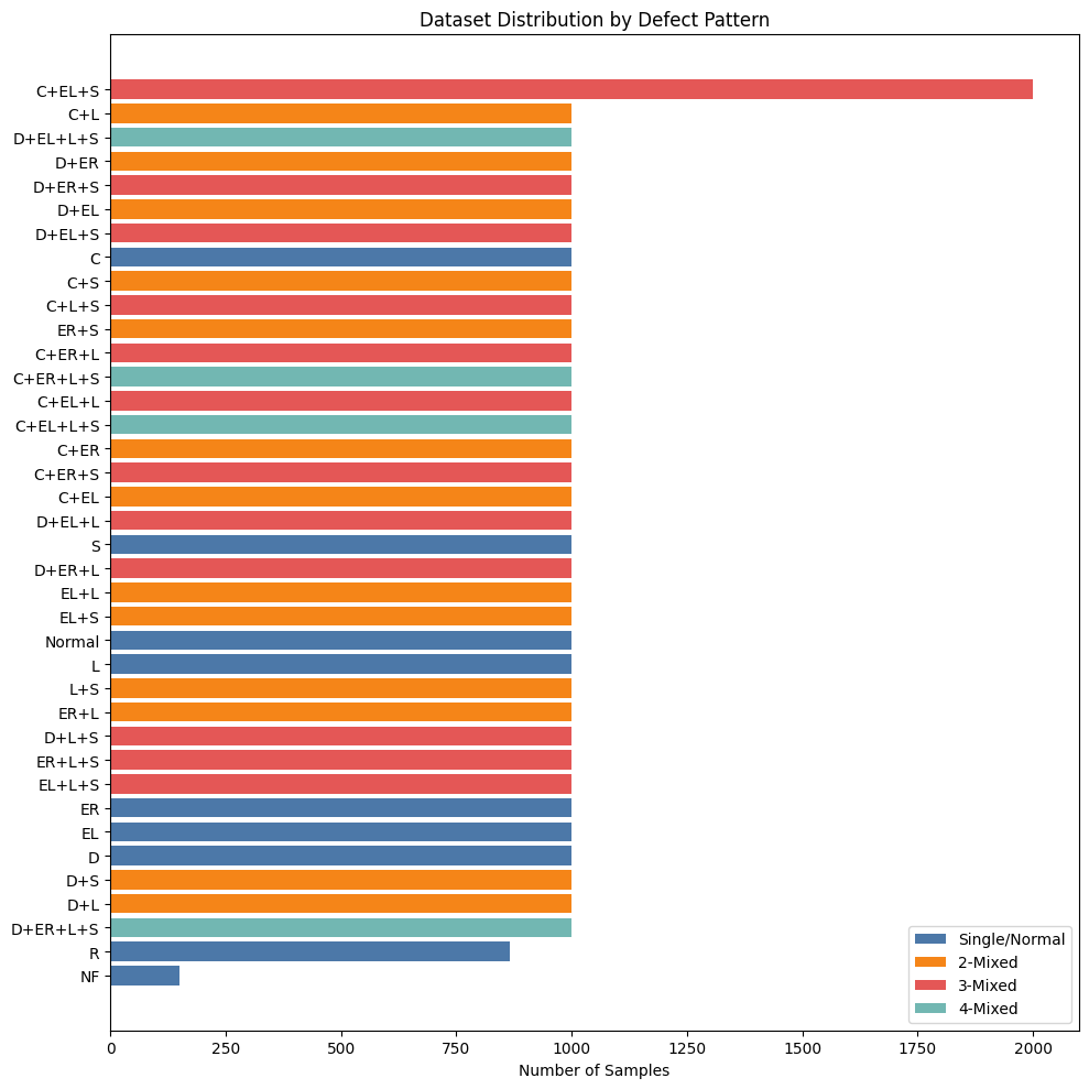
Dataset Overview

Source: Mixed-Type Wafer Map Defect Dataset

• 38,015 wafer map images
• Each image: 52 × 52 pixels
• 3 pixel states:
  • 0 = blank (no die)
  • 1 = normal die (passed test)
  • 2 = defective die (failed test)
• Labels: 8-dimensional one-hot vector (8 base defect types)
• 38 unique defect patterns (single + combinations)

Data Preprocessing Pipeline

Raw Images 52×52 Values: 0,1,2,3

→

Clean Pixel 3 → 0

→

One-Hot Encode 52×52×3 3 channels

→

Stratified Split 70 / 15 / 15

Why one-hot encode pixels? Pixel values 0, 1, 2 are categorical** (blank, normal, broken) — not ordered intensities. Treating them as numbers (0 < 1 < 2) would imply a false relationship. One-hot encoding gives each state its own channel, preserving the categorical nature.

Why only geometric augmentation? Since pixels represent discrete states (not colors), we can only apply spatial transforms** (90° rotations, flips) that don’t alter the categorical values. Color jitter or elastic deformation would corrupt the data.

Stratified Split Ensures All 38 Defect Patterns in Every Set

📦

Dataset
38 patterns
Rare (~200)

→

⚠️

Random Split
Missing patterns
in Val/Test

→

✅

Stratified Split
All 38 preserved
Train / Val / Test

Split	Samples	Unique Patterns
Train	26,610	38
Val	5,702	38
Test	5,703	38

Per-Label Sample Counts

Label	Train	Val	Test
Center	9,100	1,950	1,950
Donut	8,400	1,800	1,800
Edge_Loc	9,100	1,950	1,950
Edge_Ring	8,400	1,800	1,800
Loc	12,600	2,700	2,700
Near_Full	104	22	23
Scratch	13,300	2,850	2,850
Random	606	130	130

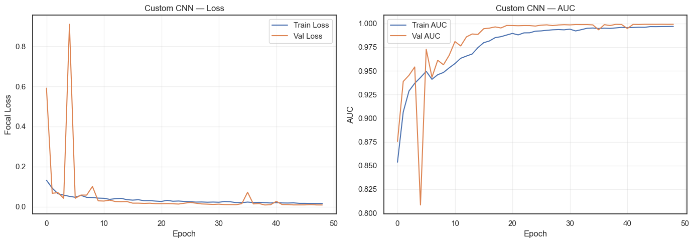
Phase 1: Detecting the 8 Base Defect Types

Output (Threshold = 50%)

Center = 80% ✅ Edge Ring = 85% ✅ Scratch = 80% ✅ Donut = 30% ❌ Edge Loc = 40% ❌ Loc = 10% ❌ Near Full = 1% ❌ Random = 23% ❌

How we validated it

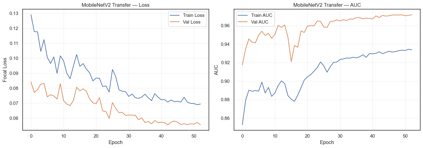
• Compared against MobileNetV2 — a model Google trained on millions of images
• If our custom model matches or beats it, we know our approach works

Custom CNN outperforms MobileNetV2

Parameter	Value	Why
Loss	Binary Focal Loss (γ=2.0)	Handles class imbalance
Optimizer	Adam (lr=1e-3)	Adaptive learning rate, fast convergence
Batch size	32	Balance between stability and speed
Epochs	Up to 100	Early stopping will cut short
ReduceLROnPlateau	patience=5, factor=0.5	Halves LR when validation plateaus
EarlyStopping	patience=10	Stops when no improvement for 10 epochs
Metrics	AUC + Binary Accuracy	AUC is threshold-independent

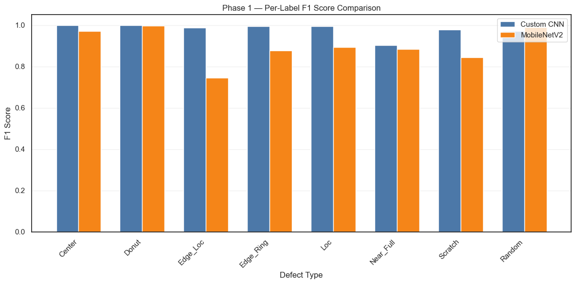
Phase 1 Results

Key observations to highlight:

• Both models achieve strong per-label F1 scores
• Near_Full is the hardest class (fewest samples ~200)
• Custom CNN and MobileNetV2 each have strengths on different defect types
• The per-label class weights in focal loss successfully boost rare-class performance

Phase 2: From 8 Base Types to 38 Defect Patterns

We take our trained Phase 1 model (which learned to detect 8 base defect types) and build on top of it to classify all 38 defect patterns.

Transfer learning from Phase 1 Model Detects 8 base defect patterns (Center, Donut, Scratch, etc.)

→

Phase 2 Model Classify all 38 defect patterns (base + combinations)

• The Phase 1 model already learned how to read wafer maps — it knows what edges, clusters, and rings look like
• We keep that knowledge and add a new layer that learns to distinguish all 38 specific patterns
• This is more efficient than training a brand new model from scratch — we’re building on what’s already been learned
• The final model picks the single most likely pattern out of 38 for each wafer

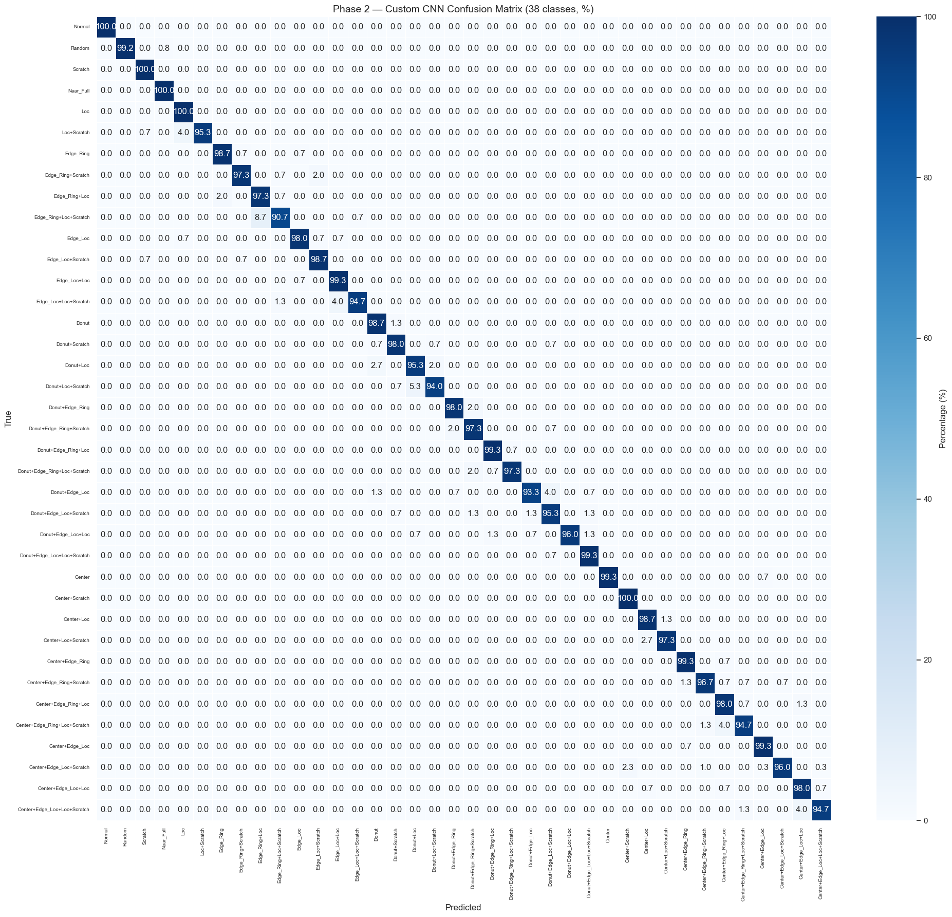
Phase 2 Results — Full Confusion Matrix (38×38)

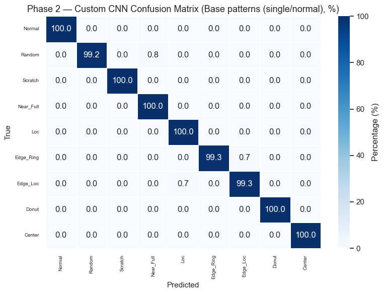
Phase 2 Results — Single / Normal Patterns

• Actual random defects are often misclassified as Near Full. These two are the low imbalance defect types.
• Edge ring and Edge loc are confused with each other.

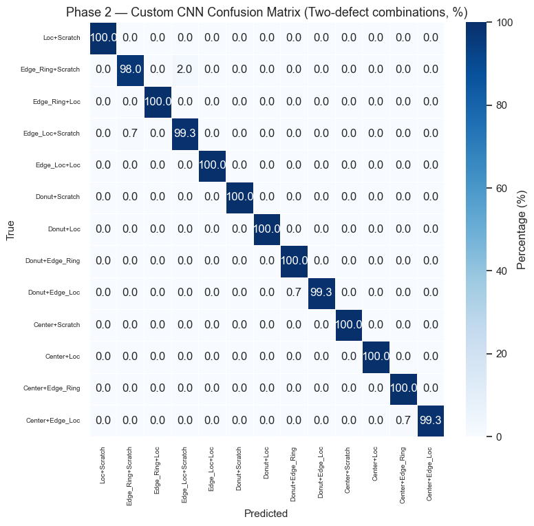
Phase 2 Results — Double Combinations

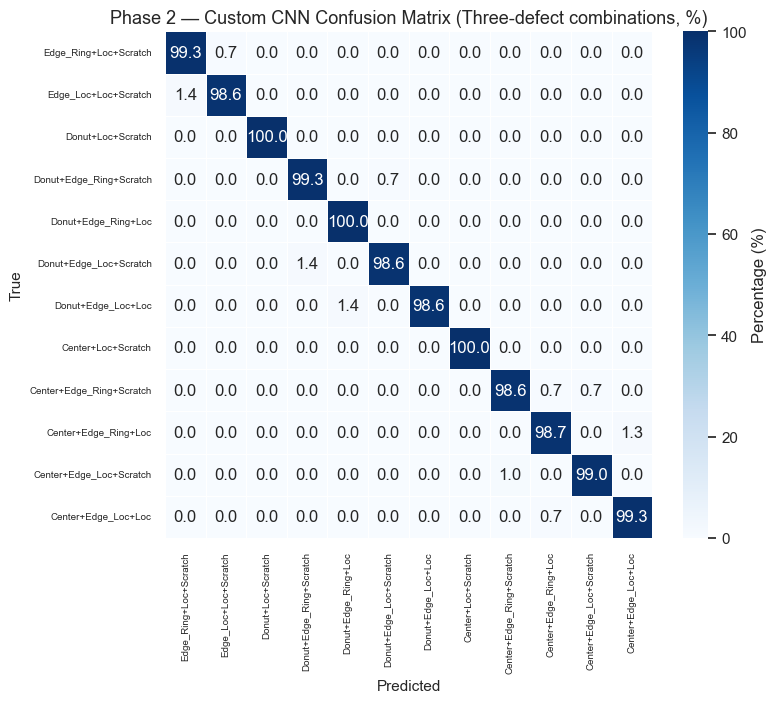
Phase 2 Results — Triple Combinations

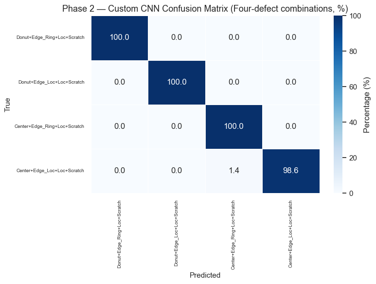
Phase 2 Results — Quadruple Combinations

Final Model Comparison

	Phase 1 — Custom CNN (8-label)	Phase 1 — MobileNetV2 (8-label)	Phase 2 — Custom CNN (38-class)	Phase 2 — MobileNetV2 (38-class)
Macro F1	0.9779	0.8998	0.9736	0.9667
Weighted F1	0.9905	0.8847	0.9735	0.9658

• Our Custom CNN outperformed MobileNetV2 in both phases
• The Phase 2 Custom CNN (38-class) is our final production model — it can identify all 38 defect patterns with 97%+ accuracy
• Building our own model from scratch proved more effective than using a pre-trained one for this task

How Accuracy is Measured

Example wafer - Center + Loc + Scratch

Phase 1: 8 Yes/No Questions Center → 90% → ✓ Yes Donut → 5% → ✗ No Edge_Loc → 3% → ✗ No Edge_Ring → 2% → ✗ No Loc → 95% → ✓ Yes Near_Full → 1% → ✗ No Scratch → 88% → ✓ Yes Random → 4% → ✗ No Above 50% = Yes, Below = No

→

Transfer Learning Freeze Phase 1 knowledge Pass features to Phase 2

→

Phase 2: Pick Best Match Center — 2% Loc+Scratch — 1% Center+Loc+Scratch — 97% Center+Scratch — 0.5% … 34 others <1% Highest probability wins

→

Accuracy Check Predicted: Center+Loc+Scratch Actual: Center+Loc+Scratch ✓ Correct

• Phase 1: Each defect scored independently — above 50% means “present.” Accuracy measured per defect type (F1 score)
• Phase 2: Picks the single highest-probability pattern out of 38. Correct if it matches the true label
• We repeat this for every wafer in the test set — 97%+ are predicted correctly

Live Inference Demo

• Dashboard link

Summary

Our Custom CNN Pipeline:

Phase 1 Train our CNN to detect 8 base defect types

→

Phase 2 Reuse Phase 1 knowledge to classify all 38 patterns

→

Final Model 38-class Custom CNN 97%+ accuracy

Benchmark Comparison:

MobileNetV2 Google’s pre-trained model (2.6M params)

→

Same tasks Phase 1 (8 types) Phase 2 (38 patterns)

→

Result Our CNN outperformed on both phases

Building our own model from scratch proved more effective than using a pre-trained one for this specialized task.

Thank You

Questions?

Appendix

The 8 Base Defect Types

Defect	Description
Center	Defects clustered at wafer center
Donut	Ring-shaped pattern in the middle
Edge_Loc	Localized defects near the edge
Edge_Ring	Defects forming a ring at the edge
Loc	Localized cluster anywhere
Near_Full	Almost entire wafer is defective
Scratch	Linear scratch pattern
Random	Randomly distributed defects

Plus Normal (no defects) and 29 combination patterns (e.g., Center+Scratch)

Key Terms

Activation Functions

• ReLU — hidden layers; if input > 0 pass through, else 0. Simple and avoids vanishing gradients
• Sigmoid — Phase 1 output; squashes to 0–1 per label. Each neuron independently says yes/no
• Softmax — Phase 2 output; converts scores to probabilities that sum to 1

Loss Functions

• Binary Focal Loss (Phase 1) — down-weights easy examples, focuses on hard/rare ones
• Sparse Categorical Crossentropy (Phase 2) — standard multi-class loss with class weights

Regularization

• Batch Normalization — normalizes layer inputs → faster, more stable training
• Dropout (0.5) — randomly silences 50% of neurons → prevents overfitting
• GlobalAveragePooling2D — averages each feature map instead of flattening → fewer parameters
• Early Stopping — stops training when validation loss plateaus
• Learning Rate - How big a step the model takes when updating its weights. Too big = overshooting; too small = too slow.

What is Transfer Learning?

Transfer learning means reusing knowledge from one task to improve performance on another.

Analogy: Imagine hiring someone who already knows how to identify shapes, edges, and textures, and just teaching them the specific wafer defect categories.

We use transfer learning twice in this project:

1. Phase 1 → Phase 2: First learn to predict the 8 base defect types, then transfer that learned knowledge to predict all 38 defect patterns
2. MobileNetV2 → Our task: Reuse a pre-trained model (trained on millions of images) as a feature extractor, and only train a new classification head on top

Two forms of transfer learning:

	From	To
Ours	Phase 1 (8 types)	Phase 2 (38 patterns)
MobileNetV2	ImageNet (millions of images)	Wafer defect classification

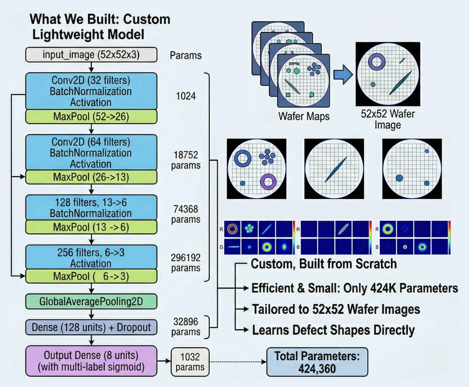
Custom CNN Architecture

Phase 1 Task: Predict which of the 8 base defect types are present (multi-label, 8 sigmoid outputs)

Model: custom_cnn — Total params: 424,264 (1.62 MB)

Layer	Shape	Params
input_image (Input)	(52, 52, 3)	0
conv2d (Conv2D)	(52, 52, 32)	896
batch_norm	(52, 52, 32)	128
activation (ReLU)	(52, 52, 32)	0
max_pooling2d	(26, 26, 32)	0
conv2d_1 (Conv2D)	(26, 26, 64)	18,496
batch_norm_1	(26, 26, 64)	256
activation_1 (ReLU)	(26, 26, 64)	0
max_pooling2d_1	(13, 13, 64)	0
conv2d_2 (Conv2D)	(13, 13, 128)	73,856

Layer	Shape	Params
batch_norm_2	(13, 13, 128)	512
activation_2 (ReLU)	(13, 13, 128)	0
max_pooling2d_2	(6, 6, 128)	0
conv2d_3 (Conv2D)	(6, 6, 256)	295,168
batch_norm_3	(6, 6, 256)	1,024
activation_3 (ReLU)	(6, 6, 256)	0
max_pooling2d_3	(3, 3, 256)	0
global_avg_pool	(256)	0
dense (ReLU)	(128)	32,896
dropout (0.5)	(128)	0
output (Sigmoid)	(8)	1,032

Design choices:

• Doubling filters (32→256): Early layers detect simple features (edges), deeper layers detect complex patterns (rings, scratches) — more filters = more capacity for complexity
• 3×3 kernels: Standard efficient choice — captures local spatial relationships
• GlobalAveragePooling over Flatten: reduces parameters from ~2,304 to 256, fighting overfitting

MobileNetV2 Architecture

Model: mobilenet_transfer — Total params: 2,587,988 (9.87 MB)

Layer	Output Shape	Params
input_image (Input)	(52, 52, 3)	0
conv2d_4 (Conv2D)	(52, 52, 3)	12
resizing (Resizing)	(224, 224, 3)	0
mobilenetv2 (Functional)	(7, 7, 1280)	2,257,984
global_average_pooling2d_1	(1280)	0
dense_1 (Dense, ReLU)	(256)	327,936
dropout_1 (Dropout)	(256)	0
output (Dense, Sigmoid)	(8)	2,056

Why MobileNetV2?

• Pre-trained on ImageNet → already knows edges, textures, shapes
• Lightweight architecture → efficient inference
• 1×1 Conv projection: Our data has 3 one-hot channels, not RGB — this layer learns the right mapping
• Frozen backbone: With only ~38K samples, fine-tuning 2.2M parameters risks overfitting

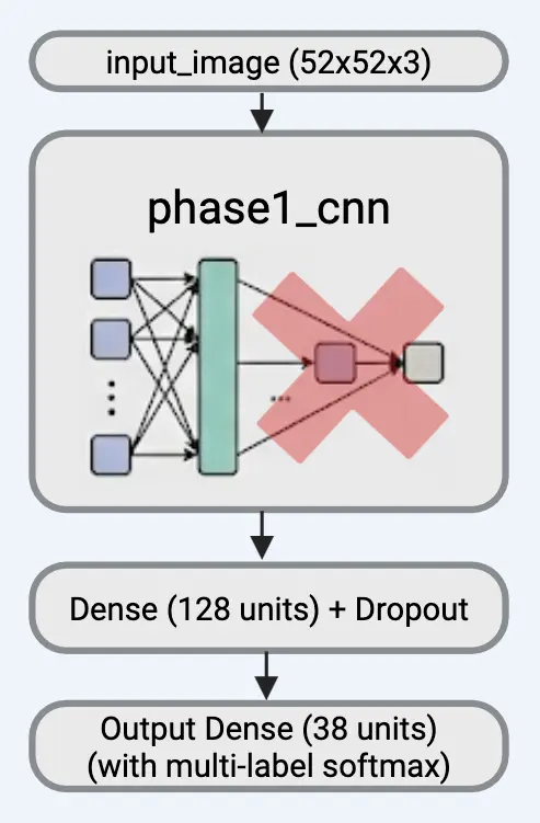
Phase 2: Two-Stage Training Details

Task: Classify each wafer into exactly one of 38 defect patterns using softmax. We reuse the Phase 1 backbone (frozen) and replace the head with Dense(128) → Dropout → Dense(38, softmax).

Stage A — Head Only Backbone: FROZEN LR: 1e-3 Epochs: ~30 Train new head only

→

Stage B — Fine-Tune Backbone: Last 25% UNFROZEN LR: 1e-5 Epochs: ~30 Fine-tune end-to-end

Why two stages?

• Stage A (head-only): The new Dense layers have random weights. Training at high LR while backbone is frozen lets them “catch up” without destroying pre-trained weights.
• Stage B (fine-tune): Unfreeze the last ~25% of backbone, train at very low LR (1e-5). Adapts features for the 38-class task while preserving prior knowledge.
• BatchNorm layers stay frozen — their statistics are from Phase 1 and shouldn’t shift.

Loss: sparse_categorical_crossentropy with balanced class weights

Model Overview

Model	Task	Output
Phase 1 — Custom CNN	8 labels	Sigmoid × 8
Phase 1 — MobileNetV2	8 labels	Sigmoid × 8
Phase 2 — Custom CNN	38 classes	Softmax × 38
Phase 2 — MobileNetV2	38 classes	Softmax × 38

Summary

What We Built

• A two-phase deep learning pipeline for wafer defect classification
• Phase 1: Multi-label detection of 8 base defect types
• Phase 2: Precise identification of all 38 defect patterns
• Two architectures: custom CNN and MobileNetV2 transfer learning

Key Technical Decisions

• One-hot pixel encoding → preserves categorical nature
• Focal Loss + class weights → handles severe imbalance
• Backbone reuse → leverages Phase 1 knowledge for Phase 2
• Two-stage fine-tuning → safe adaptation without catastrophic forgetting
• Geometric-only augmentation → respects discrete pixel states